
PIR Sensors - It's Complicated
- Graham Armitage

- May 5, 2025
- 8 min read
Abstract
The AM312 is a compact, low-power Passive Infrared (PIR) sensor widely used for motion detection in research applications, particularly small animal activity studies. Despite its advantages, the sensor exhibits performance challenges, including variations in response and delay times of single sensor and between sensors. This article examines these issues, drawing on datasheet specifications and experimental observations, to provide insigh
ts for researchers deploying the AM312 in real-world research automation applications.

Introduction
The AM312 PIR sensor is a pyroelectric sensor designed for detecting human motion through infrared radiation changes. Its small form factor (10 mm x 8 mm PCB), low quiescent current (~8–15 µA), and wide operating voltage range (2.7–12 V) make it ideal for energy-efficient applications. Despite the intended human detection it works well for detecting small warm blooded animals at close range too. This makes it popular for detecting animal movement and activity in a laboratory setting. Their low cost, availability and ease of use makes them a good choice for multi-sensor experiments by researchers.
However, practical deployment reveals challenges, including inconsistent delay times and temperature-dependent performance, which can affect reliability. This article outlines these issues, their implications, and potential mitigation strategies.
Technical Overview of the AM312
The AM312 integrates a pyroelectric element with digital signal processing, producing a high/low logic output when motion is detected. Key specifications include:
Detection Range: 3–5 meters, ~100° cone angle (lens-dependent).
Delay (hold) Time: ~2 seconds (datasheet-specified).
Blocking Time: ~2 seconds.
Operating Temperature: -20°C to +60°C.
Trigger Mode: Repeatable, maintaining high output during motion within the delay period.
These features enable standalone operation or integration with microcontrollers or other control systems. However, real-world performance often deviates from these specifications due to manufacturing variability and environmental factors.
Two terms that are crucial to research data collection are the Delay Time and Blocking Time parameters of the sensor. The delay time and blocking time of a PIR sensor, like the AM312, refer to distinct timing characteristics that govern its operation after detecting motion. Here’s a clear distinction:
Delay Time: This is the duration the sensor’s output remains high (active) after detecting motion. For the AM312, the datasheet specifies a delay time of ~2 seconds, though it can vary significantly due to manufacturing inconsistencies. During this period, the sensor signals that motion is detected, and the output stays high even if no further motion occurs. If motion persists, the delay time may extend in repeatable trigger mode.
Blocking Time: This is the duration after the delay time during which the sensor is insensitive to new motion events, effectively "locking out" further detections. For the AM312, the blocking time is also ~2 seconds, but can also vary due to manufacturing inconsistencies. During this period, the sensor ignores additional motion to prevent rapid retriggering, allowing the system to stabilize before detecting new events.
Experimental Testing
Setup
A standard factory AM312 on the factory breakout board (no additional logic circuitry) was connected to a 3.3v power supply. The output was connected directly to an oscilloscope to view and record the PIR sensor response.

A warm object was moved back and forth in front of the sensor at a distance of 15cm to simulate a small mammal in an enclosure for a typical lab setup.
The same setup and experiment was repeated with multiple sensors.
Signal Data
When the sensor detects the movement it shifts the output to a high or active state (3.3v) and after the delay time, returns to low or inactive state (0v) - assuming no movement is still being detected. The output signal is then held low by the sensor until it is ready to detect the next movement.
The object movement was deliberately started when the signal dropped low and stopped as soon as the signal went high. This was intentionally done to calculate the actual blocking time duration and delay time after movement was detected. By not continuing movement once the signal was high, the sensor delay time could also be measured.
Results
When looking at the delay time, the duration for which the signal is held high, the times varied significantly. The stated delay time from the AM312 data sheet is approximately 2 seconds. However as shown in figure 1, these delay times can be as low as 2 seconds yet can delay over 4 seconds in duration.

The blocking time, which is the time for which the sensor will not respond to movement, is quoted as approximately 2 seconds from the data sheet. Figure 2 shows that this time varied significantly from 1.7 seconds to 3.8 seconds on one example test.
When coupled with delay time, the total period of the cycle could be as high as 7.4 seconds. On average it was around 5 seconds.

Depending on the combination of the delay and blocking times, the overall period of a movement can fluctuate between 4.7 seconds and 8.4 seconds. Typically the range is within 4.8-5.2 seconds based on observations.
Performance Challenges Delay Time Variability
The AM312’s delay time, defined as the duration the output remains high after detecting motion, is specified as ~2 seconds. However, user reports indicate significant variability:
Within a Single Sensor: The tests show that significant variations occur within a single sensor, as well as between sensors even under conditions.
Between Sensors: Manufacturing inconsistencies lead to differences across units. This variability complicates applications requiring precise timing or absolute movement counts.
Implications: Inconsistent delay times can cause erratic behavior in time-sensitive applications, necessitating software adjustments or external timing circuits to stabilize output.
Constant Motion
When attempting to record continuous motion there are some approaches that can be adopted. Because the AM312 sensor remains “high” until no motion is detected, counting triggered events will not be accurate. The two main approaches are:
On Time Division: By dividing the on-time by the activity window, the number of motion events can be calculated. This requires microcontroller logic to control the output of the sensor.
Event Triggers: Adding circuitry to force retriggering and outputting a signal at regular intervals for constant motion. No microcontroller logic is needed.
Temperature Effects on Performance
PIR sensors rely on detecting infrared radiation differences, making them sensitive to ambient temperature:
Reduced Sensitivity at High Temperatures: At higher temperatures (e.g., >40°C), the contrast between human body heat and the environment decreases, reducing detection range and sensitivity. The AM312’s specified operating range (-20°C to +60°C) suggests functionality, but performance degrades near the upper limit.
False Triggers at Low Temperatures: Rapid temperature changes, such as drafts or convection near windows, can trigger false positives, as the sensor misinterprets these as motion.
Implications: Applications in environments with fluctuating temperatures (e.g., outdoor settings) require careful placement and shielding to minimize false triggers and ensure reliable detection.
No experiments to test temperature fluctuations were performed for this article.
Measuring Techniques
Two approaches can be utilized to get more consistent measurements over time.
Time Division: For ongoing movement, the total time the sensor is high, divided by the average delay time (rounded down) can derive a movement count. Because of the variability seen in the experiments, this could be erroneous. For example constant movement over 6 seconds could result in an active delay time of 9 seconds. Dividing by an average of 3 second delay time yields 3 movement counts. Fluctuations in the delay time can affect this calculation too. Because the signal remains high for continuous movement, sporadic movements at just the right time can keep the signal high for many seconds. The same movement sequence can produce different counts at different times, based on the variable cumulative delay and blocking times.
Time Interval: By setting a time window during which any activity generates a single, short high signal followed by a longer blocking time and is recorded as a single count. This can improve consistency in activity tracking. At any point during the time interval, if movement is detected, it is recorded as a single count and the remaining time in that interval is blocked. So in the above example, with a time interval of 5 seconds, a constant movement for 6 seconds would be recorded as two events.
However, if the time interval is set below the maximum delay time of the sensor, the high signal would induce a second count even if movement had stopped. For this reason, time interval values must be above the maximum delay time threshold.
To illustrate these two methods we can construct a simulation and apply both models. The first simulation is a constant motion for 12 seconds. In the second simulation, the movement occurs sporadically at 1, 7 and 12 second marks.
Figure 3 shows the simulation utilizing the Time Division method. For the constant movement simulation the AM312 could produce a 15 second or 13 second duration active signal, due to the fact that we observed variations of up to 2 seconds in the delay time. So if the movement at 12 seconds triggered the final event, it could last another 3 seconds, or the 11 second mark could have triggered the final 2 second delay.
The result is that the outcome could be 13 or 15 seconds, and applying a rounded division by 3 can yield different counts.
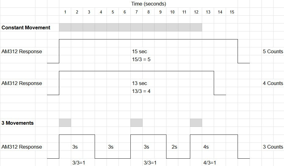
In the second simulation with discrete movements at 1,7 and 12 second marks, the AM312 could produce 3 signal events, each one being recorded as a count from division by 3. So in these 2 scenarios, it is possible to have 3 contradictory movement counts. Over time this error may cancel out or could compound, depending on the individual sensor behavior.
By repeating the same simulation, we can see very different outcomes using the time interval method in Figure 4. For the continuous movement, the circuitry with the AM312 examines the PIR state and if high produces a single 1 second signal and 4 seconds of blocking time, regardless of the actual sensor fluctuation. This produces 3 counts every time, because the maximum delay time on the PIR is below the 5 second threshold.

In the second simulation, with 3 discrete movements, each one will trigger a 1 second response. Again yielding a count of 3 movements. So both scenarios provide the same result and will continue to do so over time.
Testing the time interval method shows consistent triggers with constant movement in Figure 5. In this case approximately every 3 seconds.

Other Challenges
Blind Spots: Users report blind spots within the detection range, attributed to the small Fresnel lens.
Power Supply Noise Sensitivity: The AM312 is sensitive to power supply noise, requiring a low-noise source and additional decoupling capacitors to prevent false triggers.
Limited Output Drive: The output can only drive low-current loads (e.g., logic inputs or MOSFETs), with a 10 kΩ load reducing the output voltage from ~3 V to ~2 V, necessitating buffering for some applications.
Reflections: Infrared Radiation can be easily reflected off many surfaces. This can lead to false triggers from nearby heat sources.
Conclusion
The AM312 PIR sensor offers significant advantages for low-power, low-cost motion detection, but its performance is hampered by delay time and blocking time variability, temperature sensitivity, and other practical challenges. By understanding these issues and implementing mitigation strategies, engineers can enhance the sensor’s reliability in diverse applications.
For consistent activity measurements in a laboratory environment, clear definitions on what constitutes movement count must be determined in conjunction with the sensors used. Invariably this requires the addition of electronic circuitry to the sensor to maintain stable and consistent measurements over time.
Use of the time division method requires computational ability at the sensor to perform the math needed to derive an activity count. The time interval method will require some additional electronics, but not to the same degree of complexity making it more affordable and scalable.
Using both methods concurrently will show broad qualitative correlations but absolute or quantitative results will differ.
Comments